![]()
![]()
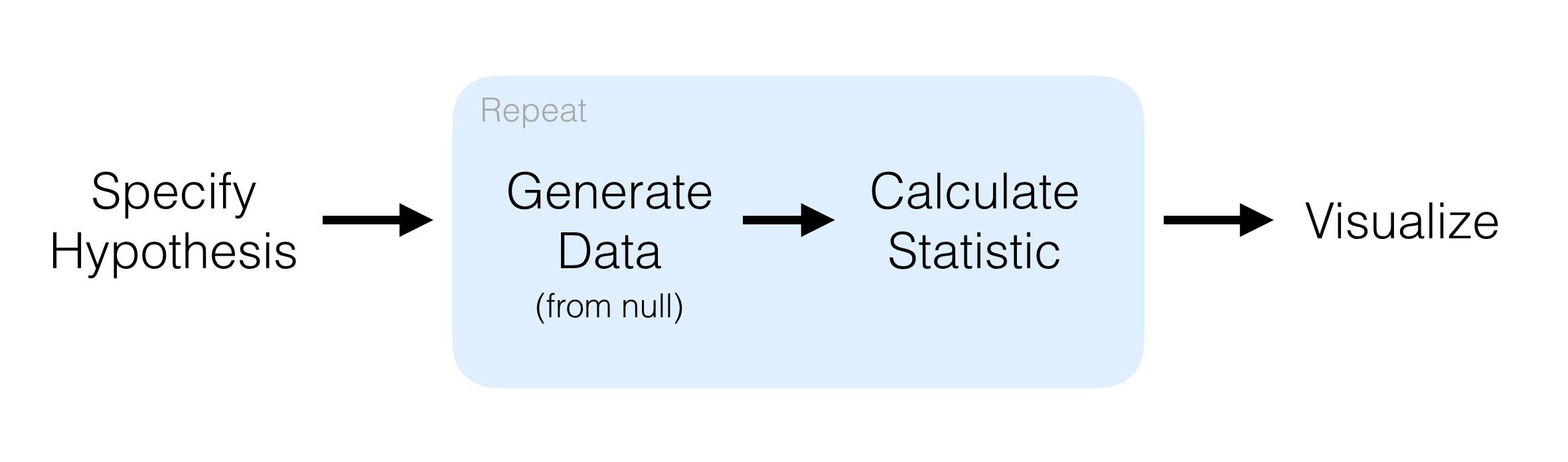
The objective of this package is to perform statistical inference using an expressive statistical grammar that coheres with the tidyverse design framework. The package is centered around 4 main verbs, supplemented with many utilities to visualize and extract value from their outputs.
-
specify()allows you to specify the variable, or relationship between variables, that you’re interested in. -
hypothesize()allows you to declare the null hypothesis. -
generate()allows you to generate data reflecting the null hypothesis. -
calculate()allows you to calculate a distribution of statistics from the generated data to form the null distribution.
To learn more about the principles underlying the package design, see vignette("infer").
If you’re interested in learning more about randomization-based statistical inference generally, including applied examples of this package, we recommend checking out Statistical Inference Via Data Science: A ModernDive Into R and the Tidyverse and Introduction to Modern Statistics.
Installation
To install the current stable version of infer from CRAN:
install.packages("infer")To install the developmental stable version of infer, make sure to install remotes first. The pkgdown website for this version is at infer.tidymodels.org.
# install.packages("pak")
pak::pak("tidymodels/infer")
Contributing
We welcome others helping us make this package as user-friendly and efficient as possible. Please review our contributing and conduct guidelines. By participating in this project you agree to abide by its terms.
For questions and discussions about tidymodels packages, modeling, and machine learning, please post on Posit Community. If you think you have encountered a bug, please submit an issue. Either way, learn how to create and share a reprex (a minimal, reproducible example), to clearly communicate about your code. Check out further details on contributing guidelines for tidymodels packages and how to get help.
Examples
These examples are pulled from the “Full infer Pipeline Examples” vignette, accessible by calling vignette("observed_stat_examples"). They make use of the gss dataset supplied by the package, providing a sample of data from the General Social Survey. The data looks like this:
## tibble [500 × 11] (S3: tbl_df/tbl/data.frame)
##  $ year   : num [1:500] 2014 1994 1998 1996 1994 ...
##  $ age    : num [1:500] 36 34 24 42 31 32 48 36 30 33 ...
##  $ sex    : Factor w/ 2 levels "male","female": 1 2 1 1 1 2 2 2 2 2 ...
##  $ college: Factor w/ 2 levels "no degree","degree": 2 1 2 1 2 1 1 2 2 1 ...
##  $ partyid: Factor w/ 5 levels "dem","ind","rep",..: 2 3 2 2 3 3 1 2 3 1 ...
##  $ hompop : num [1:500] 3 4 1 4 2 4 2 1 5 2 ...
##  $ hours  : num [1:500] 50 31 40 40 40 53 32 20 40 40 ...
##  $ income : Ord.factor w/ 12 levels "lt $1000"<"$1000 to 2999"<..: 12 11 12 12 12 12 12 12 12 10 ...
##  $ class  : Factor w/ 6 levels "lower class",..: 3 2 2 2 3 3 2 3 3 2 ...
##  $ finrela: Factor w/ 6 levels "far below average",..: 2 2 2 4 4 3 2 4 3 1 ...
##  $ weight : num [1:500] 0.896 1.083 0.55 1.086 1.083 ...
As an example, we’ll run an analysis of variance on age and partyid, testing whether the age of a respondent is independent of their political party affiliation.
Calculating the observed statistic,
Then, generating the null distribution,
null_dist <- gss |>
   specify(age ~ partyid) |>
   hypothesize(null = "independence") |>
   generate(reps = 1000, type = "permute") |>
   calculate(stat = "F")
Visualizing the observed statistic alongside the null distribution,
visualize(null_dist) +
  shade_p_value(obs_stat = F_hat, direction = "greater")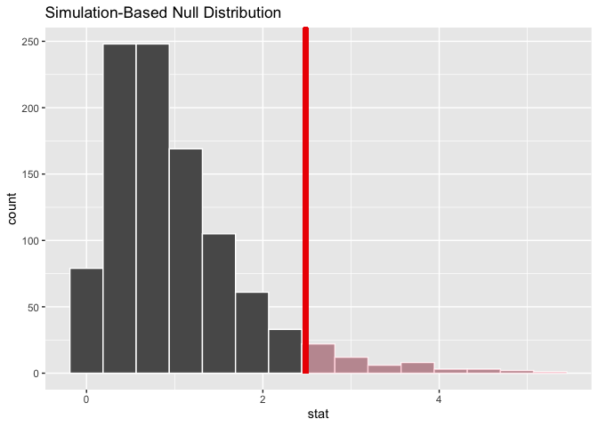
Calculating the p-value from the null distribution and observed statistic,
null_dist |>
get_p_value(obs_stat = F_hat, direction = "greater")Note that the formula and non-formula interfaces (i.e., age ~ partyid vs. response = age, explanatory = partyid) work for all implemented inference procedures in infer. Use whatever is more natural for you. If you will be doing modeling using functions like lm() and glm(), though, we recommend you begin to use the formula y ~ x notation as soon as possible.
Other resources are available in the package vignettes! See vignette("observed_stat_examples") for more examples like the one above, and vignette("infer") for discussion of the underlying principles of the package design.